
Preserve Trade Timing: Signal Smoothing Techniques Without Hand Tuning

Signal smoothing works as a low-pass filter: it strips out high-frequency noise while keeping the low-frequency pattern you actually care about. The families worth learning first are moving averages and exponential moving averages for speed, Savitzky-Golay and LOESS for preserving peak shape, median and Hampel filters for killing spikes, and Kalman or adaptive filters for data whose noise characteristics keep shifting. Every method trades noise reduction against distortion, and picking the right one starts with knowing which side of that trade-off your analysis actually needs.
TL;DR:
Moving averages and exponential moving averages are fast, simple, and suitable for long-term trend detection, but they introduce lag proportional to window size.
Savitzky-Golay filters preserve peak shape and height better than averaging methods but require careful selection of polynomial order and window length.
Kalman and adaptive filters are ideal when noise characteristics change over time, as they continuously update estimates based on a model of system dynamics.
Median and Hampel filters effectively remove spikes and outliers without blurring sharp edges, making them useful as a first line of cleanup.
Always test filters on synthetic signals, match window size to noise frequency, and consider endpoint handling to avoid artificial distortions in real-world datasets.
Table of Contents
Common Signal Filtering Techniques and When Each One Wins
Every smoother makes the same basic promise: pull a cleaner curve out of noisy data. What separates them is how they define “clean” and what they sacrifice to get there. Some techniques buy noise reduction with lag. Others buy it with computational cost. A few buys it by throwing away exactly the detail you needed.
Simple moving averages, weighted averages, and exponential moving averages form the entry point for most people learning data smoothing algorithms. A simple moving average (also called a boxcar filter) replaces each point with the average of its neighbors inside a fixed window. It’s fast, easy to explain, and easy to overdo. Widen the window and noise drops, but so does your ability to track a fast-moving trend. A weighted moving average tilts the averaging toward certain points, usually the center, so the filter responds a bit faster to real changes. The exponential moving average (EMA) skips the fixed window entirely and instead weights all past data with exponentially decaying influence, which means it reacts to new information immediately but never fully “forgets” old data. Traders and analysts favor EMA specifically because it updates continuously without needing to store a rolling buffer, a genuine advantage for streaming data.
Savitzky-Golay filters solve a specific problem that simple averaging creates: peak flattening. Instead of averaging raw values, the Savitzky-Golay method fits a low-order polynomial to a moving window of points using least-squares, then uses that polynomial to estimate the smoothed value. Because it fits curvature rather than just averaging, it tends to preserve peak height, width, and position far better than a moving average of comparable width. This matters enormously in spectroscopy, chromatography, and any dataset where the shape of a peak carries the actual information. The cost is complexity: you’re choosing both a window length and a polynomial order, and getting the order wrong (too low) reintroduces the flattening problem you were trying to avoid.
LOESS and LOWESS (locally weighted regression) extend the polynomial-fitting idea to irregularly sampled data. Rather than assuming evenly spaced points inside a fixed window, LOESS fits a weighted regression around each point using whatever neighbors happen to be nearby, weighting closer points more heavily. This flexibility makes it a strong choice when your sampling interval isn’t constant, such as sensor logs with dropped readings or financial data with gaps. The trade-off is computational cost. LOESS refits a regression at every point, which scales poorly on very large datasets compared to a simple moving average.
Median filters and Hampel filters exist for one job: killing spikes without smearing the rest of the signal. A median filter replaces each point with the median of its local window instead of the mean, which means a single wild outlier gets ignored rather than dragged into the average. This preserves sharp edges and step changes that a moving average would blur. The Hampel filter goes a step further, only replacing a point when it deviates from the local median by more than a set number of standard deviations, leaving everything else untouched. That selectivity makes Hampel filtering a preferred first pass before applying a smoother, since it removes bad data points without touching legitimate variation.
Gaussian, triangular, and binomial filters produce smoother impulse responses than a plain boxcar. Where a moving average has hard edges (every point in the window counts equally, then suddenly not at all), a Gaussian filter tapers its weighting so points near the center of the window matter more than points at the edges. This produces less ringing and a more natural-looking curve. There’s a neat shortcut here: applying a simple boxcar smooth multiple times in a row approximates a Gaussian shape at a fraction of the computational cost, a technique worth knowing if you’re smoothing large volumes of data in real time.
Kalman filters and other adaptive filters depart from fixed-window thinking entirely. Instead of applying the same rule to every data point, an adaptive filter estimates a system’s state and continuously updates its own parameters based on incoming measurements and a model of how the system evolves. This makes Kalman filtering the right call for genuinely nonstationary data, where the noise level or the underlying process itself changes over time. It also asks more of you: you need at least a rough model of the underlying dynamics, which raw averaging methods never require.
Quick reference for matching technique to goal:
Trend detection over long time frames: moving average or EMA
Preserving peak height and shape: Savitzky-Golay
Irregular sampling or need for flexible local fitting: LOESS/LOWESS
Removing spikes while keeping edges sharp: median or Hampel filter
Smooth impulse response, low computational cost: Gaussian or multi-pass boxcar
Changing noise statistics, online estimation: Kalman or adaptive filter
There’s no single best smoothing algorithm; the right pick always depends on what you’re trying to protect in the underlying signal.
How Do You Choose the Right Smoothing Method?
Start with a question most people skip: what am I actually trying to preserve? Trend detection, transient preservation, and outlier removal each point toward a different filter, and guessing without answering this first is how people end up smoothing away the exact feature they needed.
Here’s a working checklist for narrowing down your choice:
Define the goal first. Are you looking for a slow-moving trend, trying to keep a sharp transition intact, or hunting for isolated bad data points? Each goal rules out entire families of techniques.
Estimate your acceptable lag. Wider windows cut more noise but respond more slowly to real changes. If your application needs near-real-time response (live sensor dashboards, trading signals), a heavy moving average will frustrate you before it helps you.
Pick an odd window width for symmetric filters. An odd-numbered window keeps a center point exactly in the middle, which prevents the output from shifting peak positions left or right relative to the input. This is a small detail with an outsized effect on anything involving peak timing.
Decide whether outliers exist in your data before you smooth. If spikes are present, run a median or Hampel filter first. Applying a moving average directly to spiky data smears the spike across neighboring points instead of removing it.
Check whether your noise statistics are stationary. If noise levels change across your dataset (louder during certain hours, quieter during others), a fixed-window filter will be under-tuned somewhere. That’s your signal to look at Kalman or adaptive filtering instead.
Test on a synthetic step or impulse signal. Before trusting a filter on real data, run it on an artificial step function and a single spike. Watching how the filter responds to these idealized inputs tells you exactly how much lag and peak distortion to expect on real data.
The window-versus-lag trade-off deserves its own callout because it’s the single most common mistake in practical signal smoothing: people default to a wide window because it “looks cleaner” on a chart, without noticing they’ve delayed every real signal change by half the window width.
Pro Tip: Run the same dataset through two or three window widths side by side before committing to one. If the pattern you care about survives a much narrower window, you’re probably over-smoothing and adding unnecessary lag for no real noise benefit.
For choosing between families: reach for Savitzky-Golay or LOESS when the shape and position of local features (peaks, curves, inflection points) matter to your downstream analysis. Reach for median or Hampel filtering when your main enemy is a handful of bad readings rather than continuous background noise. Reach for Kalman filtering only when you have reason to believe the noise itself is changing character over time, since setting one up properly requires more modeling work than a simple moving average.
Avoiding Endpoint Errors and Multi-Pass Smoothing Mistakes
Smoothing algorithms look clean in textbooks and get messy at the edges of real datasets. Two problems show up constantly: what happens at the start and end of your data, and what happens when you apply a smoother more than once.
Endpoint handling trips up more analyses than any other implementation detail. A centered moving average needs data on both sides of each point, which is a problem at the very first and last points in your dataset, since there’s no “before the start” or “after the end” data to average in. Common fixes include padding the edges with repeated boundary values, trimming the unusable edge points entirely, or switching to a one-sided (causal) filter that only looks backward. That last option matters more than it sounds: a causal filter is the only kind usable in real-time applications, since a non-causal filter needs future data points that haven’t happened yet. If you’re building anything that reacts to live data as it arrives, you need a causal design, and you should accept the extra lag that comes with it.
Resampling and periodic noise interact in a way that catches people off guard. If your data contains a strong periodic noise component, such as electrical line noise at a known frequency, a moving average whose window length happens to match (or badly mismatch) that period can either cancel the noise cleanly or reinforce it. Before choosing a moving average length, check whether your data has a dominant periodic component and size the window accordingly, or resample first to remove the ambiguity.
Multi-pass smoothing follows a specific combination rule worth memorizing: running a boxcar smooth of width w a total of n times produces an effective window of n × w − n + 1 points, according to Terpconnect’s smoothing reference. Three passes of a 5-point smooth, for instance, behave like a much wider single-pass filter, and the resulting shape approaches a Gaussian curve. That’s a genuinely useful shortcut for cheap Gaussian-like smoothing, but each additional pass adds more lag to the step response, so it’s not free.
Practical notes worth keeping in your back pocket:
Choose window widths based on the noise frequency you’re trying to remove, not by trial and error on a chart that “looks nice.”
Always test parameter choices against a synthetic step function to see the actual step response before trusting it on production data.
For large datasets or streaming pipelines, EMA and simple moving averages scale far better than LOESS or full Kalman implementations, since they don’t require refitting a model at every point.
Cross-validation works for selecting smoothing parameters when you have enough data to hold some out, but heuristic rules of thumb (like matching window width to known noise periods) are often good enough in practice.
When Fixed Filters Fall Short: Kalman and Adaptive Methods
Fixed-window filters assume the world stays the same shape it was when you tuned them. Real data rarely cooperates that way. That gap is exactly what Kalman filters and adaptive filtering were built to close.
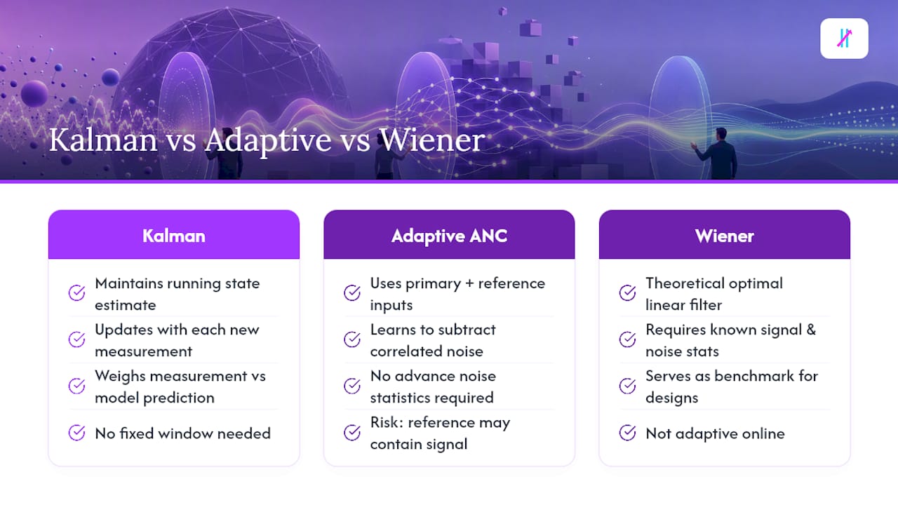
A Kalman filter maintains a running estimate of a system’s state, then updates that estimate every time a new measurement arrives, weighing the new data against the filter’s own prediction based on a model of how the system should behave. This makes it a natural fit for state-estimation problems, tracking a moving object’s position, estimating a sensor’s true reading under variable noise, or following a trend that speeds up and slows down unpredictably. Unlike a moving average, a Kalman filter doesn’t need a fixed window; it updates continuously and can adjust how much it trusts new measurements versus its own prediction.
Adaptive noise cancellation takes a related but distinct approach. Instead of modeling the signal’s dynamics directly, it uses a primary input (the signal you want, contaminated with noise) and a separate reference input that’s correlated with the noise but ideally uncorrelated with the desired signal itself. The adaptive filter learns, in real time, how to subtract the noise captured in the reference channel from the primary signal. This technique, first formalized by Widrow and colleagues at Stanford, remains a foundational reference for engineers building adaptive systems that must work without prior knowledge of the noise characteristics.
The Wiener filter serves as the theoretical benchmark against which adaptive designs are measured. It represents the mathematically optimal linear filter for separating signal from noise when you know the statistics of both in advance. Adaptive filters approximate this optimum without needing that advance knowledge, learning the right parameters as data arrives instead.
The real risk with adaptive noise cancellation is contamination of the reference channel. If the reference input picks up any of the actual desired signal, not just the noise, the adaptive filter will partially cancel your real signal along with the noise you wanted removed. That’s a subtle failure mode that won’t show up as an obvious error; your output will simply look cleaner and smaller than it should. The practical trigger for switching from a fixed smoother to an adaptive one is straightforward: if your noise level or character visibly changes across your dataset (louder in some regimes, quieter in others), a fixed filter tuned for one condition will underperform somewhere else, and that’s your cue to invest the extra setup work.
What Are Smoothing Splines and When Should You Use Them?
A smoothing spline takes a different philosophical approach than any window-based filter. Instead of processing data locally point by point, it fits one continuous analytic function to the entire dataset, balancing two competing goals: staying close to the actual data points and staying smooth (avoiding sharp wiggles). That balance is controlled by a penalty parameter, often called lambda or s, that determines how much smoothness you’re willing to trade for fit accuracy. Push the penalty toward zero and the spline interpolates every data point exactly, noise included. Push it higher and the curve flattens toward something closer to a simple trend line.
SciPy offers several smoothing-spline routines that differ mainly in how they define and default that penalty. make_smoothing_spline and make_splrep use different penalty formulations and default behaviors, while the older UnivariateSpline interface offers a more manual approach to setting the smoothness factor directly. The differences matter mostly at the boundaries of your data and in how aggressively each function’s defaults smooth without any tuning at all, so it’s worth testing more than one on a small sample before committing.
Splines earn their place over window filters in three specific situations: irregularly sampled data where a fixed window doesn’t make geometric sense, situations where you need an actual analytic function (for computing derivatives cleanly, for instance, rather than just smoothed sample values), and multi-dimensional smoothing where fitting a continuous surface beats stitching together separate 1D filters.
Selecting the smoothing parameter itself is its own small project. Generalized cross-validation (GCV) offers a principled, data-driven way to pick a penalty automatically by minimizing prediction error on held-out points. Absent that, a reasonable heuristic is to start with a low penalty, visually inspect how much noise remains, and increase it gradually until the curve stops changing shape between adjustments.
Practical Examples: MATLAB, SciPy, and Quick Recipes to Try
Theory only gets you so far. Here’s what to actually type.
In MATLAB, four functions cover most day-to-day smoothing needs. movmean computes a simple moving average over a specified window. movmedian does the same job with a median instead of a mean, which is your go-to when spikes are present. smoothdata acts as a general-purpose wrapper that can apply moving average, Gaussian, or Savitzky-Golay smoothing depending on the method argument you pass it. sgolayfilt runs a dedicated Savitzky-Golay implementation where you specify both polynomial order and window length directly. MathWorks’ signal smoothing examples walk through parameter choices for each, including how resampling interacts with moving-average length and how a Hampel filter step can clean data before a final smoothing pass.
In Python, SciPy’s make_smoothing_spline and make_splrep handle spline-based smoothing, while UnivariateSpline gives more direct manual control over the smoothness factor. For window-based approaches, scipy.signal.savgol_filter implements Savitzky-Golay filtering directly, and scipy.ndimage.median_filter handles spike removal.
A short recipe checklist to run through on any new dataset:
Plot the raw signal first and visually identify whether spikes, gradual noise, or both are present.
If spikes exist, apply a median or Hampel filter as a first pass before anything else.
Try a moving average or EMA with two or three different window widths, plotted together, to see the lag-versus-smoothness trade-off directly.
If peak shape matters, run Savitzky-Golay with a modest polynomial order (2 or 3) and compare against the moving average result.
Test your final choice against a synthetic step function to confirm the step response and lag match what your application can tolerate.
Check residuals (raw minus smoothed) for remaining structure. Genuine noise residuals should look random; if you see leftover pattern, your smoother didn’t remove what it should have.
How We Apply Smoothing to Trading Signals
Raw price and indicator data is jittery by nature, and that jitter is exactly what generates false signals when you’re trying to time an entry or exit. At Big Move Algo, smoothing exists to clarify trend direction without erasing the timing information that actually matters for a trade decision. That’s a narrower goal than general-purpose data cleaning: a trader doesn’t just want a smoother line, they need the smoothed line to still tell them the right moment to act.
Peak and step-change timing is where most naive smoothing approaches fail traders. A heavily smoothed moving average might look clean on a chart, but if it delays a genuine trend reversal by several bars, that lag directly costs entry price. This is why preserving the precise timing of transitions matters more in trading applications than in most other smoothing use cases.
Our Fake Trend Detector works alongside smoothing rather than replacing it, filtering out choppy, low-quality conditions where even a well-tuned smoother would still generate misleading signals. As a general rule, intraday signals benefit from shorter, more responsive smoothing windows to keep pace with faster price action, while swing signals can tolerate wider windows since the trend they’re tracking unfolds over more bars. Neither setting is fixed; both should be evaluated against the specific market and timeframe you’re trading, similar to the regime filtering approach we’ve written about separately.
A Final Word on Choosing the Right Approach
The biggest mistake I see people make with signal smoothing techniques isn’t picking the “wrong” algorithm. It’s skipping the step of defining what they’re actually trying to protect in the data before they touch a single parameter. A trend detector and a peak-preservation tool solve different problems, and no amount of parameter tuning fixes a fundamentally mismatched technique.
Always plot the raw signal against the smoothed output before trusting it. Test at least two or three window widths side by side. Pay close attention to what happens at the edges of your dataset, since endpoint artifacts quietly distort more analyses than people realize. Run your chosen filter against a synthetic step or spike input first. If it behaves the way you expect there, it will behave the way you expect on the real thing.
— Steven Hartwell
A Ready-Made Option for Traders Who Don’t Want to Hand-Tune Filters
Building and validating your own smoothing pipeline, testing window widths, checking step response, tuning a Hampel threshold, takes real time most traders would rather spend watching the market. Big Move Algo packages that filtering work into a TradingView indicator that hands you a clear Long, Short, or Exit signal instead of a raw noisy chart you have to interpret yourself.

AUTO Mode applies the built-in smoothing and trend logic with minimal setup, so you get structured signals without configuring a single filter parameter. Manual Mode opens up customization for traders who want to adjust sensitivity themselves, and the Fake Trend Detector screens out the choppy, low-quality conditions where even a carefully tuned smoother tends to mislead. The indicator runs across crypto, forex, stocks, indices, and commodities, works on unlimited devices, and includes free updates as the underlying logic improves.
Plans start at $55 per month or $660 per year for Version 2, with Version 3 and Version 3 Plus available at higher tiers for traders who want additional features. Check current pricing and feature details to find the version that matches how you trade.
Sources
FAQ
What Are Smoothing Techniques and What Are They Used For?
Smoothing techniques reduce high-frequency noise in a dataset while preserving the underlying low-frequency pattern, effectively acting as a low-pass filter. They’re used to clarifying trends, remove sensor jitter, prepare data for peak detection, and make patterns easier to see or analyse downstream.
What Are Some Common Methods for Smoothing Data?
The most widely used data smoothing algorithms are moving averages (simple, weighted, and exponential), Savitzky-Golay filters, LOESS/LOWESS local regression, median and Hampel filters, Gaussian filters, and Kalman or adaptive filters. Each fits a different goal, from long-term trend tracking to spike removal to nonstationary noise handling.
What Are the Different Types of Smoothing Techniques?
Smoothing techniques generally split into fixed-window filters (moving average, Gaussian, Savitzky-Golay), robust outlier-focused filters (median, Hampel), curve-fitting approaches (smoothing splines, LOESS), and adaptive methods (Kalman filters, adaptive noise cancellation) that adjust their own parameters as data arrives.
How Do I Know Which Signal Filtering Technique to Use?
Start by defining whether you need trend detection, transient preservation, or outlier removal, since each goal favors a different family of techniques. Test your candidate filter against a synthetic step or spike signal first to see its actual lag and distortion before applying it to real data.
Does Big Move Algo Handle Signal Smoothing Automatically?
Yes. Big Move Algo applies built-in smoothing and trend logic through its AUTO Mode, and its Fake Trend Detector filters out choppy, low-quality market conditions that would otherwise generate unreliable signals. Manual Mode is available for traders who want to adjust that filtering themselves.
Recommended
Comments